Unsupervised Learning with Linear Algebra

The following snippet will help us to reload the source .py file into our notebook whenever we make updates.

%load_ext autoreload
%autoreload 2

# %reload_ext autoreload

Link to Source Code

Hereis a link to the source code for this post.

Link to reference for this blog post

Here is a link to the main reference we use as we implement this post.

Now, let’s begin!

Part I: Image Compression with the Singular Value Decomposition

We use the image of a cat which can be accessed here for free download: www.pexels.com. I have already downloaded a copy of an image of a tabby cat, and I have stored it in the same directory as this jupyter notebook.

Our main work horse for Image Compression is Singular Value Decomposition, but before we introduce that, let’s recall a few definitions and facts from linear algebra. First, let \(A\) be a \(m\times n\) matrix. Let’s consider the matrix \(A^TA\), which is \(n\times n\) and symmetric, because \((A^TA)^T\) is still \(A^TA\). Now, we recall that if \(\lambda\) is an eigenvalue of \(A^TA\), then \(\lambda \geq 0\). This is a fact from linear algebra, and let’s just take it as given here. Now, let \(\lambda_1, \lambda_2, \cdots, lambda_n\) denote the eigenvalues of \(A^TA\), allowing repetitions. We could assume we have ordered them so that \(\lambda_1 \geq \lambda_2 \geq \lambda_3, \cdots \geq 0\). Now let \(\sigma_i = \sqrt{\lambda_i},\) and you guessed it, the numbers \(\sigma_{1} \geq \sigma_{2} \geq \cdots \geq \sigma_{n}\) are the singular values of \(A\).

Let \(A\) be an \(m\times n\) matrix with singular values \(\sigma_{1} \geq \sigma_{2} \geq \cdots \geq \sigma_{n} \geq 0\), Let \(r\) denote the number of nonzero singular values of \(A\), or equivalently the rank of \(A\). Then, the singular value decomposition of \(A\) is a factorization \[ A = U \Sigma V^T \] where \(U\) is a \(m \times m\) orthogonal matrix, \(V\) is a \(n \times n\) orthogonal matrix, and \(\Sigma\) is an \(m \times n\) matrix whose \(i\) th diagonal entry equals the \(i\) th singular value \(\sigma_{i}\) for \(i = 1,\cdots, r\). All other entries of \(\Sigma\) are zero.

We won’t go into detail about how the decomposition is actually computed, since we will focus on the implementation and application to compressing images, which roughly speaking, is about storing the image as a fraction of the original size, while still maintain a reasonable level of image resolution or sharpness so that we did not sacrafice too much image quality to store it with a reduced size.

from matplotlib import pyplot as plt
import numpy as np
np.random.seed(42)
import PIL
from PIL import Image
import urllib
import networkx as nx
from sklearn.neighbors import NearestNeighbors
from sklearn.metrics import pairwise_distances
def read_image(url):
    return np.array(PIL.Image.open(urllib.request.urlopen(url)))
# url = "https://images.pexels.com/photos/1170986/pexels-photo-1170986.jpeg?cs=srgb&dl=pexels-evg-kowalievska-1170986.jpg&fm=jpg"
# myimg = read_image(url)

After loading in the required packages, let us read in the tabby_cat.png image we have already downloaded to our current directory. We could get some information about this file right-away by running the following code snippet:

# open the image from working directory
img = Image.open("./tabby_cat.png")
print(f"format: {img.format}")
print(f"size: {img.size}")
print(f"mode: {img.mode}")
# convert PIL images into numpy arrays.
myimg = np.asarray(img)

format: JPEG
size: (1771, 2657)
mode: RGB

We see that our image is of dimension \(1771 \times 2657\), and it is a color image, as denoted by \(RGB\). For the purpose of this blog post, we would like to work with grayscale images so let us turn it into grayscale with the following code, and plot the original image and the grayscale one side-by-side. We see the color image on the left and the gray-scale image on the right. Great job!

fig, axarr = plt.subplots(1, 2, figsize = (7, 3))

def to_greyscale(im):
    return 1 - np.dot(im[...,:3], [0.2989, 0.5870, 0.1140])

grey_img = to_greyscale(myimg)

axarr[0].imshow(myimg)
axarr[0].axis("off")
axarr[0].set(title = "original")

axarr[1].imshow(grey_img, cmap = "Greys")
axarr[1].axis("off")
axarr[1].set(title = "greyscale")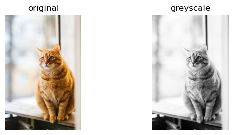

Actually, before we lauch into the implementation of SVD, let us do an example to calculate the SVD of a 2 by 2 matrix by hand, so we know what’s going on exactly.

Let \(A\) be the matrix \[ A = \begin{bmatrix} 3 & 0\\ 4 & 5\\ \end{bmatrix} \] Let’s find \(U\). We have
\[ A^T = \begin{bmatrix} 3 & 4\\ 0 & 5\\ \end{bmatrix} \] Thus \[ A A^T = \begin{bmatrix} 9 & 12\\ 12 & 41\\ \end{bmatrix} \] Now we find the eigenvalue and eigenvectors of \(AA^T\) by computing \[ det(AA^T -I \lambda) =0 \] We get the characteristic function \(\lambda^2 - 50 \lambda + 225 = 0\). We could factor it into linear factors, and we get \[ (\lambda - 45)(\lambda - 5) = 0 \] so \(\lambda_1 = 45,\) and \(\lambda_2 = 5\). For eigenvalue \(45\), the eigenvector is \((1,3)^T\), and for eigenvalue \(5\), the eigenvector is \((3,-1)^T\). Hence, we get \[ U = \frac{1}{\sqrt{10}} \cdot \begin{bmatrix} 1 & 3\\ 3 & -1\\ \end{bmatrix} \] Now, since eigenvalues of \(AA^T\) equals the eigenvalues of \(A^TA\), we could get our singular values. \(\sigma_1 = \sqrt{\lambda_1} = \sqrt{45}\), and \(\sigma_2 = \sqrt{\lambda_2} = \sqrt{5}\). Hence, we get \[ \Sigma = \begin{bmatrix} \sqrt{45} & 0\\ 0 & \sqrt{5}\\ \end{bmatrix} \] Note that the order of the singular value need to match the eigenvectors in \(U\) we got earlier. Now, we need to get \(V\). We obtain this by calculating the eigenvalue and eigenvectors of \(A^TA\), and since it’s similar to before, let’s just write down the answer here. \[ V= \frac{1}{\sqrt{2}} \begin{bmatrix} 1&1\\ 1&-1\\ \end{bmatrix} \] Now, after seeing this example, we feel we have a better understanding of SVD decomposition. Hence, let us return to our cat image.

We see that we have successfully turned our cat image to greyscale, and it is represented in the python notebook as numpy array. Let’s check the dimension of this array once more just to be sure.

print(grey_img.shape[0])
print(grey_img.shape[1])

2657
1771

We have introduced the concept of singular value decompostion, but how do we compute it? If we want to compute it by hand, then there are quite a few mathematical steps to follow. However, for the purpose of this blog, we just need to use the following numpy snippet: U, sigma, V = np.linalg.svd(A). And we will get the matrices U, sigma, and V returned to us as numpy arrays. This numpy function is very useful, and it helped us a great deal in our implementation of image processing, which now import.

from hidden_images import svd
svd1 = svd()

The main thing we implemented is a function called reconstruct() that takes an image (represented as a numpy array), use np.linalg.svd() to perform the singular decomposition on it, then we truncate the singular values and only use the first \(k\) of them, so we use index slicing to obtain the truncated version of V, Sigma, and U, and we multiply them together again to obtain the reconstructed image, which takes up less storage. If we pick a small number of singular values, i.e., a small \(k\), our picture will look like it has pretty low resolution. The picture below on the left shows the original image, and the picture on the right shows the reconstructed image, which in this case, has a reasonable resolution, since we selected a relatively sizable \(k=18\).

As for how to do the numpy array slicing to only use the first \(k\) singular values, we could use the following code snippet as shown in the main reference we have listed under ### Source. Let us attach an underscore _ to the letter denoting we have truncated this matrix.

U_ = U[:,:k] means we take the first \(k\) columns of \(U\) to form U_.

D_ = D[:k, :k] means we take the upper left \(k\times k\) square matrix from \(D\) to form D_.

V_ = V[:k,:] means we take the first \(k\) rows from \(V\) to form V_.

k = 18 
A_ = svd1.reconstruct(grey_img, k)
svd1.compare_images(grey_img, A_)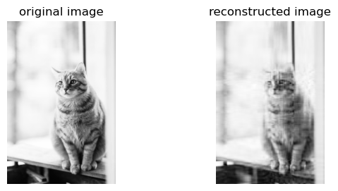

Now, we perform an experiment, which is implemented in the experiment function. Basically, we start with using only \(3\) singular values, and we increase the number of ingular values by \(5\) each time, until the reconstructed image looks roughly the same just from looking at it. Meanwhile, as we print out these images, we also print a string showing how much storage (in percentage of the original picture) that our reconstructed image takes up.

svd1.experiment(grey_img)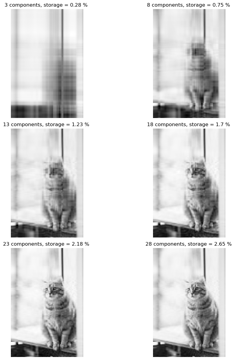 

We see that at \(28\) singular values, our reconstructed picture of the cat already looks pretty much the same as the orignal image, albeit slightly grainy. However, the exciting thing is that now, we only need \(2.65\) percent of the original storage space for this reconstructed image! So we sacrifice a little image sharpness, and greatly reduce the storage we needed to store this image!

Part II: Spectral Community Detection

We would like to use Laplacian spectral clustering algorithm to find clusters in data sets represented as a graph. First, what do we mean by graphs? Mathematically, graphs is a tuple \((V,E)\) where \(V\) is a set of vertices, or nodes, and elements in \(E\) are subsets of \(V\) that represent edges. Hence, the element in set \(E\) are themselves sets of elements of \(V\)! That’s a mouthful, but we are not going to deal with these, let us just plot a graph to see for ourselves. Also, notice that in networkx package, we could use different layouts for plotting our graphs.

import matplotlib.pyplot as plt
fig, ax = plt.subplots(figsize = (6, 3))
import networkx as nx
G = nx.petersen_graph()
subax1 = plt.subplot(131)
nx.draw(G) # spring_layout
subax2 = plt.subplot(132)
nx.draw(G, pos=nx.circular_layout(G), node_color="r", edge_color="b")
subax3 = plt.subplot(133)
nx.draw_spectral(G)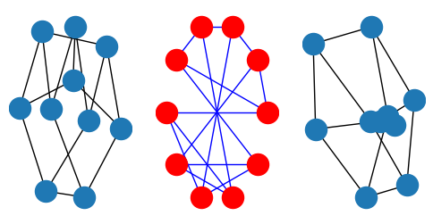

Now we know what a graph looks like, we would like to talk a little about clustering data using Laplacian Spectral clustering. Basically, clustering is a form of unsupervised learning where our goal is to group data points into “related” groups. For example, in the below plot, we could see clearly that there are two “blobs” of data, each blob is a cluster. The clustering task is identify clusters that fits the data, even when we do not have any labels y. Sometimes, we just need to eyeball the data and say, well, it seems we should classify the data into these two clusters!

from sklearn.datasets import make_blobs
fig, ax = plt.subplots(1, figsize=(3,3))
X,y = make_blobs(n_samples=100, n_features=2, centers=2, random_state=1)
a=ax.scatter(X[:,0], X[:,1])
a=ax.set(xlabel="feature 1", ylabel="feature 2")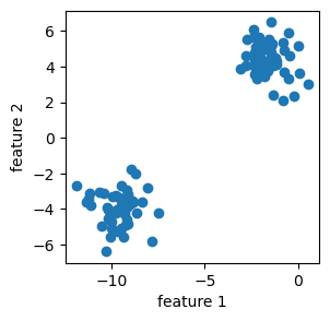

Now, laplacian spectral clustering is a method that use matrix eigenvectors to cluster data. It’s most effective for binary clustering, and it works for nonlinear clustering of data.

Here’s a road map: first, we need to compute the \(k\)-nearest-neighbors graph using NearestNeighbors from sklearn.neighbors. Then we define a clustering to be good if it does not “cut” too many edges. An edge is “cut” if it has two nodes in different clusters. However, one can always minimize cut by assigning all the vertices of the graph to the same label! Hence, we label the whole graph as a single cluster, which is not terribly interesting. Thus, we need to normalize the cut. Thus, we need concepts such as the volume of a cluster, and the normalized cut objective function.

Implementing Laplacian Spectral Clustering

from sklearn.datasets import make_blobs, make_circles
from matplotlib import pyplot as plt
import numpy as np
np.random.seed(42)

We are interested in using Laplacian spectral clustering to cluster the two circles into their own clusters.

np.random.seed(42)

n = 500
X, y = make_circles(n_samples=n, shuffle=True, noise=0.07, random_state=None, factor = 0.5)

fig, ax = plt.subplots(1, figsize = (4, 4))
a = ax.scatter(X[:, 0], X[:, 1])
a = ax.set(xlabel = "Feature 1", ylabel = "Feature 2")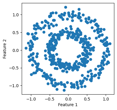

Now, let us see NearestNeighbors at work in the following cell.

from sklearn.neighbors import NearestNeighbors

k = 10
nbrs = NearestNeighbors(n_neighbors=k).fit(X)
A = nbrs.kneighbors_graph().toarray()

# symmetrize the matrix
A = A + A.T
A[A > 1] = 1

Let us import the spectral python class that we implemented. We could use the plot_graph function we implemented in there to plot the nearest neighbor graph for us.

import networkx as nx
from hidden_spectral import spectral 
spec  = spectral()
plt.rcParams["figure.figsize"] = (4,4)
spec.plot_graph(X, A)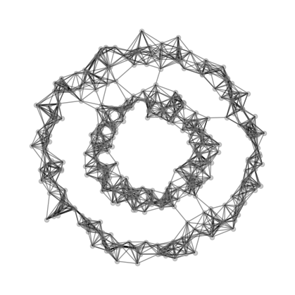

# fig, axarr = plt.subplots(1, 2, figsize = (8, 4))
y_bad = np.random.randint(0, 2, n)
# plot_graph(X, A, z = y, ax = axarr[0])
# plot_graph(X, A, z = y_bad, ax = axarr[1])

Here’s now volume of a cluster \(j\) in matrix \(A\) with clustering vector \(z\) is defined: \[ vol_j (A,z) = \sum_{i=1}^{n} \sum_{k=1}^{n} \mathbb{1}[z_i = j]a_{ik} \] We could think of \(vol_j(A,z)\) as representing the number of edges that have one node in cluster \(j\). Now, the normalized cut objective function is \[ f(z,A) = cut(A,z) (1/vol_0(A,z) + 1/vol_1(A,z)) \] It turns out that we are not going to use these equations directory in our actual implementation, and instead, we’ll use approximated versions of these functions.

from sklearn.neighbors import NearestNeighbors
from sklearn.metrics import pairwise_distances
def cut(A, z):
    D = pairwise_distances(z.reshape(-1, 1))
    return (A*D).sum()
    
print(f"good labels cut = {cut(A, z = y)}") 
print(f"bad labels cut = {cut(A, z = y_bad)}") 

def cut(A, z):
    D = pairwise_distances(z.reshape(-1, 1))
    return (A*D).sum()
    
print(f"good labels cut = {cut(A, z = y)}") 
print(f"bad labels cut = {cut(A, z = y_bad)}") 

good labels cut = 22.0
bad labels cut = 3000.0
good labels cut = 22.0
bad labels cut = 3000.0

Use theorems from linear algebra

Hence, let \(z \in \{0,1\}^n\) denote the binary vector that we try to predict, then we form a \(\~{z}\) such that \[ \~{z_i} = 1/vol_0(A,z) \ \text{when} \ z_i = 0 \] and \[ \~{z_i} = 1/vol_1(A,z) \ \text{when} \ z_i = 1 \] Now, our objective function becomes \[ f(z) = \frac{\~{z}^T (D-A)\~{z}} {\~{z}^T D \~{z}} \] where \(D\) is a diagonal matrix with \(\sum_{i=1}^n a_{ij}\) on the j-th position on the diagional. We are omitting many mathematical steps here, but that is okay, since we do not need to know all these details when we implement this in code. What we do need is the result from doing all these computations: \(z\) turns out to be the eigenvector with the second smallest eigenvalue of the matrix \[L = D^{-1}\left[ D-A \right]. \] This matrix \(L\) is called the normalized Laplacian. Hence, this equation about \(L\) is all we need to turn into code for our implementation to work.

from hidden_spectral import spectral 
spec = spectral()
fig, ax = plt.subplots(figsize = (4, 4))
z_ = spec.second_laplacian_eigenvector(A=A)
spec.plot_graph(X, A, z=z_, ax = ax, show_edge_cuts = False)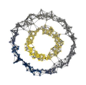

We see that our plots looks good! Our code distinguishes the inner ring from the outer ring, successfully classifying them into different clusters! Below, we also highlight the cut edges.

z = z_ > 0
fig, ax = plt.subplots(figsize = (4, 4))
spec.plot_graph(X, A, z, show_edge_cuts = True, ax = ax)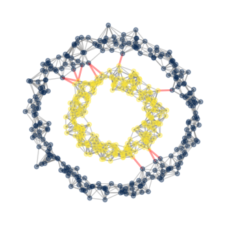

Let us try our implementation on a different data set.

from sklearn.datasets import make_moons

H, z = make_moons(n_samples=100, random_state=1, noise = .1)
fig, ax = plt.subplots(figsize = (4, 4))
a = ax.scatter(H[:, 0], H[:, 1])
a = ax.set(xlabel = "Feature 1", ylabel = "Feature 2")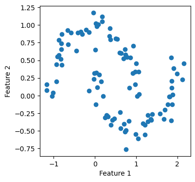

Again, our implementation worked! Now, we want to experiment a little with how big a value we should pick for n_neighbors, which is the number of neighbors needed to form the nearest-neighbors graph. This is a parameter that requires some fine-tuning. Hence, let us try several values and see how each of them performs.

fig, ax = plt.subplots(figsize = (4, 4))
z_hat = spec.spectral_clustering(H, k=6)
a = ax.scatter(H[:, 0], H[:, 1], c = z_hat, cmap = plt.cm.cividis)
a = ax.set(xlabel = "Feature 1", ylabel = "Feature 2")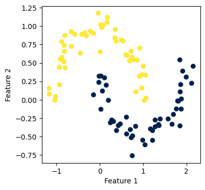

fig, axarr = plt.subplots(2, 3, figsize = (6, 4))

i = 2
for ax in axarr.ravel():
    z = spec.spectral_clustering(X, k = i)
    a = ax.scatter(X[:, 0], X[:, 1], c = z, cmap = plt.cm.cividis)
    a = ax.set(xlabel = "Feature 1", ylabel = "Feature 2", title = f"{i} neighbors")
    i += 1

plt.tight_layout()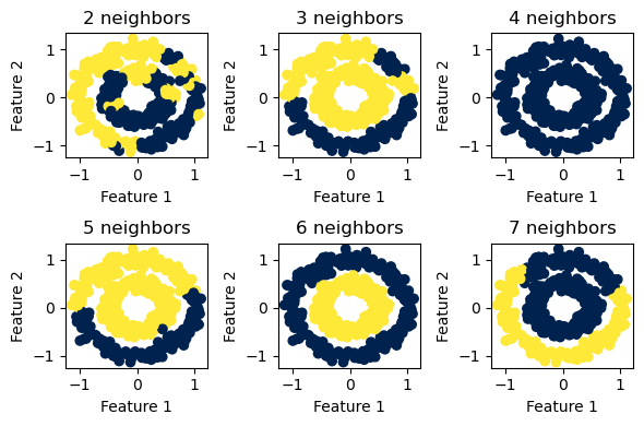

We see that for the two concentric circles, \(6\) neighbors seems to be the sweet spot.

fig, axarr = plt.subplots(2, 3, figsize = (6, 4))

i = 2
for ax in axarr.ravel():
    z = spec.spectral_clustering(H, k = i)
    a = ax.scatter(H[:, 0], H[:, 1], c = z, cmap = plt.cm.cividis)
    a = ax.set(xlabel = "Feature 1", ylabel = "Feature 2", title = f"{i} neighbors")
    i += 1

plt.tight_layout()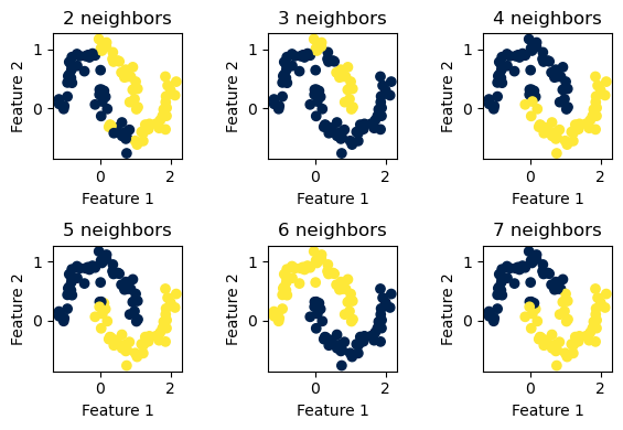

For the two “half-moon” shapes, \(6\) neighbors again seems to be the optimal value to use.

Now, since we have a working Laplacian spectral clustering implementation, let us try it on a classic graph for community detection.

Evaluate the Laplacian spectral clustering algorithm on the “Karate Club Graph”

Now it’s time to test whether our implementation of spectral clustering is doing a good job at community detection or not! Let us import the networkx library and plot the Karate Club Graph, where each node (dot/vertex) represents a member of a karate club. Edges in this graph represents social ties between two club members. We could think of it this way: if there is an edge between two members, we assume those two members had a good time together in the karate club. Let’s plot the graph and see how it looks like.

We see that there seems to be two “clusters” in the graph, one around node \(0\), which is the instructor of the club, “Mr. Hi”, and another around node \(33\), which is the club president. Assume that this graph is going to split into two graphs, one around node \(0\) and one around node \(33\), representing the split up of the actual club into two separate clubs. Could our implementation predict the division of the graph based solely on the social ties, which are edges, that we see here in the graph? Let’s find out!

import networkx as nx
G = nx.karate_club_graph()
layout = nx.layout.fruchterman_reingold_layout(G)
nx.draw(G, layout, with_labels=True, node_color = "steelblue")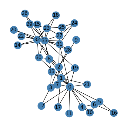

clubs = nx.get_node_attributes(G, "club")
G_np = nx.to_numpy_array(G)
z_hat = spec.spectral_clustering(G_np, k=6)
print(type(z_hat.tolist()))

<class 'list'>

print(clubs)
keys = range(34)
z_hat_list = z_hat.tolist()
mydict = dict(zip(keys, z_hat_list))
print(mydict)

{0: 'Mr. Hi', 1: 'Mr. Hi', 2: 'Mr. Hi', 3: 'Mr. Hi', 4: 'Mr. Hi', 5: 'Mr. Hi', 6: 'Mr. Hi', 7: 'Mr. Hi', 8: 'Mr. Hi', 9: 'Officer', 10: 'Mr. Hi', 11: 'Mr. Hi', 12: 'Mr. Hi', 13: 'Mr. Hi', 14: 'Officer', 15: 'Officer', 16: 'Mr. Hi', 17: 'Mr. Hi', 18: 'Officer', 19: 'Mr. Hi', 20: 'Officer', 21: 'Mr. Hi', 22: 'Officer', 23: 'Officer', 24: 'Officer', 25: 'Officer', 26: 'Officer', 27: 'Officer', 28: 'Officer', 29: 'Officer', 30: 'Officer', 31: 'Officer', 32: 'Officer', 33: 'Officer'}
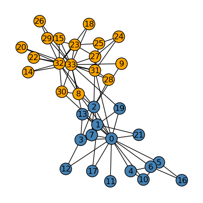
{0: 0, 1: 0, 2: 0, 3: 0, 4: 0, 5: 0, 6: 0, 7: 0, 8: 1, 9: 1, 10: 0, 11: 0, 12: 0, 13: 0, 14: 1, 15: 1, 16: 0, 17: 0, 18: 1, 19: 0, 20: 1, 21: 0, 22: 1, 23: 1, 24: 1, 25: 1, 26: 1, 27: 1, 28: 1, 29: 1, 30: 1, 31: 1, 32: 1, 33: 1}

Below, we see that our implementation did a good job splitting the graph into two “clusters”, or “communities”, that more or less fits our imagination if we eyeball the graph.

nx.draw(G, layout,
        with_labels=True, 
        node_color = ["steelblue" if mydict[i] == 0 else "orange" for i in mydict.keys()],
        edgecolors = "black" # confusingly, this is the color of node borders, not of edges
        ) 

Now, we compare the performance between our implementation (above) and the actual splitting of the graph (below).

nx.draw(G, layout,
        with_labels=True, 
        node_color = ["orange" if clubs[i] == "Officer" else "steelblue" for i in G.nodes()],
        edgecolors = "black" # confusingly, this is the color of node borders, not of edges
        ) 

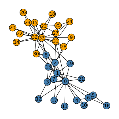
We see that our implementation of community detection differs from the original club split by one node, namely, node \(8\). Hence, overall, our implementation of spectral_clustering performed really well.

Appendix: Source Code

The Python source files used in this post are reproduced below so that readers of the rendered site can inspect the implementation without needing access to the underlying repository.

hidden_images.py

from matplotlib import pyplot as plt
import numpy as np
np.random.seed(42)


class svd:
    def __init__(self) -> None:
        self.sigma = None
        self.svdSize = None
        
    def reconstruct(self, img: np.array, k: int):
        U, self.sigma, V = np.linalg.svd(img)
        # create the Sigma matrix in the SVD
        Sigma = np.zeros_like(img,dtype=float) # matrix of zeros of same shape as matrix img 
        Sigma[:min(img.shape),:min(img.shape)] = np.diag(self.sigma)        # singular values on the main diagonal

        # pick first k col of U
        # pick top k singular values of Sigma
        # pick first k row of V
        if (k <= img.shape[0]) and (k <= img.shape[1]):
            U_ = U[:,:k]
            Sigma_ = Sigma[:k, :k]
            V_ = V[:k, :]
            A_ = U_ @ Sigma_ @ V_
            U_size = U_.shape[0] * U_.shape[1]
            V_size = V_.shape[0] * V_.shape[1]
            Sigma_size = Sigma_.shape[0] * Sigma_.shape[1]
            self.svdSize = U_size + V_size + Sigma_size
            return A_



    def experiment(self, img):
        fig, axarr = plt.subplots(3, 2, figsize = (12, 12))
        n_pixel_img = (img.shape[0] * img.shape[1])
        i = 3 
        for ax in axarr.ravel():
            A_ = self.reconstruct(img, i)
            n_pixel_A_ = self.svdSize 
            storage = ( n_pixel_A_ / n_pixel_img ) * 100
            storage = round(storage, 2)
            ax.imshow(A_, cmap = "Greys")
            ax.axis("off")
            ax.set(title = f"{i} components, storage = {storage} % ")
            i += 5 

        plt.tight_layout()

    def compare_images(self, A: np.array, A_: np.array) -> None:

        fig, axarr = plt.subplots(1, 2, figsize = (7, 3))

        axarr[0].imshow(A, cmap = "Greys")
        axarr[0].axis("off")
        axarr[0].set(title = "original image")

        axarr[1].imshow(A_, cmap = "Greys")
        axarr[1].axis("off")
        axarr[1].set(title = "reconstructed image")

        
            

hidden_spectral.py

from sklearn.datasets import make_blobs, make_circles
from matplotlib import pyplot as plt
import numpy as np
import numpy.linalg as linalg
import networkx as nx
from sklearn.neighbors import NearestNeighbors
from sklearn.metrics import pairwise_distances

class spectral:
    def __init__(self) -> None:
        self.L = None
        self.D = None
        self.X = None

    def cut(self, A, z):
        D = pairwise_distances(z.reshape(-1, 1))
        return (A*D).sum()

    def vol(self, j, A, z):
        return A[z == j,:].sum()

    def normcut(self, A, z):
        return self.cut(A, z) * (1/self.vol(0, A, z) + 1/self.vol(1, A, z))

    def second_laplacian_eigenvector(self, A: np.array) -> np.array:
        self.D = np.diag(A.sum(axis = 0))
        # print(self.D)
        self.L = np.linalg.inv(self.D) @ (self.D-A)
        # print(self.L)
        evalue, evector = np.linalg.eig(self.L)
        k = self.L.shape[1] 
        idx = evalue.argsort()[:k][::-1] 
        evalue = evalue[idx]
        evector = evector[:, idx]
        # access eigenvector associated with the second smallest eigenvalue 
        index = evector.shape[1]
        return evector[:, index-2] 



    def spectral_clustering(self, X, k = 6) -> np.array:
        nbrs = NearestNeighbors(n_neighbors=k).fit(X)
        A = nbrs.kneighbors_graph().toarray()
        A = A + A.T
        A[A > 1] = 1
        z = self.second_laplacian_eigenvector(A)
        # convert floats to 0s and 1s, so we just have two colors when we plot it.
        z = 1 * (z>0)
        return z 



    def plot_graph(self, X, A, z = None, ax = None, show_edge_cuts = True):
        G = nx.from_numpy_array(A)
        if z is None:
            nx.draw(G, pos = X, alpha = .4, node_color = "grey", node_size = 20, ax = ax)
        else: 
            if show_edge_cuts:
                colors = ["red" if z[i] != z[j] else "grey" for i, j in G.edges()]
                widths = [2 if z[i] != z[j] else 1 for i, j in G.edges()]
            else:
                colors = "black"
                widths = 1
            
            nx.draw(G, pos = X, alpha = .4, node_color = z, node_size = 20, edge_color = colors, width = widths, ax = ax, cmap=plt.cm.cividis)

        plt.gca().set(xlabel = "Feature 1", ylabel = "Feature 2")



'''
Recorded here for testing
'''
# L = np.diag([4,5,22,2,3])
# # print(L)
# evalue, evector = np.linalg.eig(L)
# print("evalue")
# print(evalue)
# print("evector")
# print(evector)
# k = L.shape[1] 
# idx = evalue.argsort()[:k][::-1] 
# evalue = evalue[idx]
# evector = evector[:, idx]

# print("evalue after change")
# print(evalue)
# print("evector after change")
# print(evector)

# index = evector.shape[1]
# print("col")
# print(evector[:,index-2])