import forwardprocess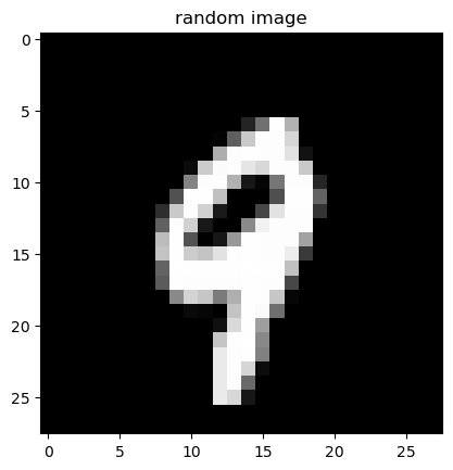
This report documents an end-to-end PyTorch implementation of the Denoising Diffusion Probabilistic Model (DDPM) introduced by Ho, Jain, and Abbeel (2020). After a self-contained derivation of the forward and reverse diffusion processes, we walk through every component of the implementation: the linear \beta variance schedule, the closed-form forward marginal q(x_t \mid x_0), the noise-prediction reparameterization \epsilon_\theta, and the time-conditional U-Net built from residual blocks, self-attention, and sinusoidal time embeddings. We train the model on the MNIST handwritten-digit dataset and present qualitative samples produced by the trained network.
Diffusion-based generative models – DDPM (Ho, Jain, Abbeel 2020), score-based models (Song & Ermon 2019), latent diffusion (Stable Diffusion), Imagen, DALL-E 2 – are now the dominant paradigm for high-quality image synthesis. They have eclipsed earlier approaches such as GANs and pixel-CNNs because they are simple to train (a single regression-style objective), stable (no adversarial game), and capable of remarkably high sample quality.
A diffusion model has two parts:
The forward process needs no learning – it is a hand-designed Gaussian Markov chain. All of the modelling effort goes into the reverse process, where a neural network \epsilon_\theta(x_t, t) is trained to predict the noise that was added to a clean image at timestep t. Once trained, the network is plugged into a standard sampling loop to generate new images.
This project evolves out of investigating a problem from MATH 649 Deep Learning at Texas A&M University, which I took in Spring 2025. > Problem: Design, implement, and train a diffusion model on the > MNIST dataset of handwritten images. Sample from the generative model > and examine what the samples look like.
We follow the algorithms from the paper Denoising Diffusion Probabilistic Models by Ho, Jain, and Abbeel (2020), and rely heavily on the expositions in The Annotated Diffusion Model by Niels Rogge and Kashif Rasul, and Diffusion Models from Scratch by Michael Wornow.
The project has three goals:
diffusers, transformers, or other high-level libraries – just torch, torchvision, numpy, and matplotlib.The remainder of the report is organised as follows. §2 sets up the forward process and the closed-form identity that makes diffusion training tractable. §3 visualises the forward process on a real MNIST digit. §4 derives the noise-prediction reparameterization and the L_\text{simple} objective, then walks through the training loop. §5 walks through the sampling loop. §6 dissects the U-Net used as \epsilon_\theta. §7 covers dataset, hyperparameters, and the training run. §8 presents qualitative samples. §9 discusses results, limitations, and possible extensions.
| File | What it contains |
|---|---|
helper.py |
Hyperparameters; \beta_t, \alpha_t, \bar\alpha_t, \sigma_t schedules; sinusoidal time embedding; the sampling loop; small utilities. |
forwardprocess.py |
Stand-alone script that loads MNIST, picks one digit, and visualises the forward process. |
main.py |
Training driver: loads MNIST, builds the model, trains, and saves the checkpoint. |
loadmodel.py |
Loads a checkpoint and runs the sampling loop to generate sample trajectories. |
model.py |
The time-conditional U-Net (Model). |
resnetblock.py |
The ResnetBlock building block (used inside the U-Net). |
attnblock.py |
Self-attention block over spatial positions. |
downsample.py, upsample.py |
The 2\times down- and up-sampling blocks. |
We model the data distribution as q(x_0) and treat a real sample x_0 \sim q(x_0) as the starting point of a T-step Markov chain. The transition kernel is a fixed conditional Gaussian:
q(x_t \mid x_{t-1}) = \mathcal{N}\!\bigl(x_t;\ \sqrt{1 - \beta_t}\, x_{t-1},\ \beta_t I\bigr),
parameterised by a known variance schedule 0 < \beta_1 < \beta_2 < \dots < \beta_T < 1. Each step rescales the previous image by \sqrt{1 - \beta_t} and adds isotropic Gaussian noise with variance \beta_t. In code we sample from this kernel via the reparameterization trick:
x_t \;=\; \sqrt{1 - \beta_t}\, x_{t-1} \;+\; \sqrt{\beta_t}\, \epsilon, \qquad \epsilon \sim \mathcal{N}(0, I).
The schedule is chosen so that, after T steps, x_T has effectively forgotten x_0 and is approximately distributed as \mathcal{N}(0, I). We use the same simple linear schedule as the paper, but with a smaller number of timesteps suitable for 28 \times 28 MNIST images:
# helper.py
T          = 50
betas      = torch.linspace(1e-4, 1e-1, T)
alphas     = 1 - betas
alpha_bars = torch.Tensor(np.cumprod(alphas))
sigmas = torch.sqrt(betas)Naively, sampling x_t requires running t Markov-chain steps. Fortunately, because the chain is Gaussian, we can collapse all t steps into a single closed-form expression. Define
\alpha_t \;=\; 1 - \beta_t, \qquad \bar\alpha_t \;=\; \prod_{s=1}^{t} \alpha_s.
Two observations are enough to derive the closed form. First, repeated application of the reparameterization formula gives
x_t = \sqrt{\alpha_t}\, x_{t-1} + \sqrt{1 - \alpha_t}\,\epsilon_t = \sqrt{\alpha_t \alpha_{t-1}}\, x_{t-2} + \sqrt{\alpha_t (1 - \alpha_{t-1})}\,\epsilon_{t-1} + \sqrt{1 - \alpha_t}\,\epsilon_t,
with all \epsilon_s independent standard normals. Second, the sum of two independent zero-mean Gaussians with variances a and b is itself a zero-mean Gaussian with variance a + b. Applying these two facts t times collapses everything to
\boxed{\quad q(x_t \mid x_0) \;=\; \mathcal{N}\!\bigl(x_t;\ \sqrt{\bar\alpha_t}\, x_0,\ (1 - \bar\alpha_t) I\bigr). \quad}
Equivalently,
x_t \;=\; \sqrt{\bar\alpha_t}\, x_0 \;+\; \sqrt{1 - \bar\alpha_t}\,\epsilon, \qquad \epsilon \sim \mathcal{N}(0, I). \tag{$\star$}
This identity is the workhorse of training: it lets us jump directly from x_0 to any x_t in a single line of code, instead of unrolling the full Markov chain. Because \bar\alpha_t shrinks toward zero as t \to T, the signal \sqrt{\bar\alpha_t}\, x_0 vanishes and the noise \sqrt{1 - \bar\alpha_t}\,\epsilon takes over, yielding x_T \approx \mathcal{N}(0, I) as desired.
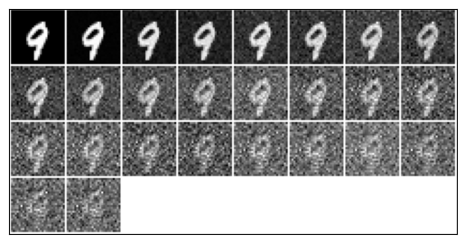
To get an intuition for what the forward process does to a real image, we apply it to a randomly chosen MNIST digit. The cell below imports forwardprocess.py, which:
random.seed(42)).The first figure below is the clean digit x_0; the second figure is the entire noising trajectory.
# forwardprocess.py (relevant part)
def fwd_process(x_0):
    T = 25
    betas = torch.linspace(1e-4, 1e-1, T)
    x_ts, x_t_1 = [], x_0
    for t in range(T):
        epsilon = torch.randn(x_0.shape)
        beta_t  = betas[t]
        x_t = x_t_1 * np.sqrt(1 - beta_t) + epsilon * np.sqrt(beta_t)
        x_ts.append(x_t)
        x_t_1 = x_t
    show_image([x_0] + x_ts)
import forwardprocess
The first figure is the clean image x_0 – a randomly drawn MNIST digit. The second figure is a strip of T + 1 = 26 thumbnails ordered left-to-right: the leftmost is again x_0, and each subsequent thumbnail is one further step along the forward Markov chain. Visually, the digit fades into a structureless cloud of Gaussian static. By the right end of the strip we have effectively destroyed all signal – exactly the regime x_T \approx \mathcal{N}(0, I) predicted by the closed-form (\star) above.
This visualisation makes clear why we cannot simply subtract noise with a hand-coded rule: at intermediate timesteps the image is already corrupted enough that neural-network-level pattern recognition is needed to recover any plausible underlying digit. That is precisely the job of \epsilon_\theta in the next section.
The forward kernel q(x_t \mid x_{t-1}) is fixed, but the corresponding posterior q(x_{t-1} \mid x_t) – needed to actually undo a noising step – is intractable in closed form because it requires marginalising over x_0. Conditioned on x_0, however, a clean Gaussian posterior exists:
q(x_{t-1} \mid x_t, x_0) \;=\; \mathcal{N}\!\bigl(x_{t-1};\ \tilde\mu_t(x_t, x_0),\ \tilde\beta_t I\bigr),
with
\tilde\mu_t(x_t, x_0) \;=\; \frac{\sqrt{\bar\alpha_{t-1}}\,\beta_t}{1 - \bar\alpha_t}\, x_0 \;+\; \frac{\sqrt{\alpha_t}\,(1 - \bar\alpha_{t-1})}{1 - \bar\alpha_t}\, x_t, \qquad \tilde\beta_t \;=\; \frac{1 - \bar\alpha_{t-1}}{1 - \bar\alpha_t}\,\beta_t.
We approximate the unknown q(x_{t-1} \mid x_t) with a parameterised Gaussian
p_\theta(x_{t-1} \mid x_t) \;=\; \mathcal{N}\!\bigl(x_{t-1};\ \mu_\theta(x_t, t),\ \Sigma_\theta(x_t, t)\bigr).
Following Ho et al. (2020) we fix the variance \Sigma_\theta = \sigma_t^2 I – the paper compares \sigma_t^2 = \beta_t and \sigma_t^2 = \tilde\beta_t; we use \sigma_t = \sqrt{\beta_t} – and only learn the mean \mu_\theta.
Solving the closed-form identity (\star) for x_0 in terms of \epsilon gives
x_0 \;=\; \frac{1}{\sqrt{\bar\alpha_t}}\bigl(x_t - \sqrt{1 - \bar\alpha_t}\,\epsilon\bigr).
Substituting this into the expression for \tilde\mu_t(x_t, x_0) and simplifying yields the equivalent expression
\tilde\mu_t(x_t, x_0) \;=\; \frac{1}{\sqrt{\alpha_t}}\!\left(x_t - \frac{\beta_t}{\sqrt{1 - \bar\alpha_t}}\,\epsilon\right).
This motivates parameterising \mu_\theta in the same form, but with a learned noise prediction \epsilon_\theta(x_t, t) in place of the unknown \epsilon:
\boxed{\quad \mu_\theta(x_t, t) \;=\; \frac{1}{\sqrt{\alpha_t}}\!\left(x_t - \frac{\beta_t}{\sqrt{1 - \bar\alpha_t}}\,\epsilon_\theta(x_t, t)\right). \quad}
So instead of asking the network to produce a denoised image directly, we ask it to predict the noise component \epsilon that was added to x_0 to obtain x_t. This is the central modelling choice of DDPM, and it is what turns variational inference on a deep latent-variable model into something that looks like ordinary supervised regression.
The full variational lower bound on \log p_\theta(x_0) decomposes into a sum of KL divergences, one per timestep. Substituting the Gaussian forms above and discarding terms that do not depend on \theta (and ignoring constant prefactors that depend only on t), the per-timestep objective collapses to
L_\text{simple}(\theta) \;=\; \mathbb{E}_{t,\,x_0,\,\epsilon}\!\left[\, \bigl\lVert \epsilon - \epsilon_\theta\!\bigl(\sqrt{\bar\alpha_t}\, x_0 + \sqrt{1 - \bar\alpha_t}\,\epsilon,\; t\bigr)\bigr\rVert^{2} \,\right].
This is just a mean-squared error between the true noise \epsilon and the network’s prediction. It has none of the moving pieces of GAN training (no discriminator, no adversarial game, no mode-collapse pathologies); it is a single regression loss, which is one of the reasons DDPMs are so well-behaved in practice.
The expectation in L_\text{simple} is estimated by stochastic gradient descent. At each step we sample one (or one minibatch of) clean images x_0, sample a uniform timestep t, sample fresh Gaussian noise \epsilon, and update \theta by taking a gradient step on the squared error between \epsilon and \epsilon_\theta.

main.pyEach line of the algorithm has a one-line counterpart in our train function. The loop body, lightly reformatted:
# main.py (excerpt from `train`)
for batch_idx, (x_0, _) in enumerate(trainloader):
    B = x_0.shape[0]
    x_0 = x_0.to(model.device)                            # x_0 ~ q(x_0)
    t = torch.randint(0, T, (B,))                         # t ~ Uniform({0, ..., T-1})
    epsilon = torch.randn(x_0.shape, device=model.device) # epsilon ~ N(0, I)

    # x_t ~ q(x_t | x_0) using the closed form (*)
    x_0_coef     = torch.sqrt(alpha_bars[t]).reshape(-1, 1, 1, 1).to(model.device)
    epsilon_coef = torch.sqrt(1 - alpha_bars[t]).reshape(-1, 1, 1, 1).to(model.device)
    x_t = x_0_coef * x_0 + epsilon_coef * epsilon

    epsilon_theta = model(x_t, t.to(model.device))        # network prediction
    loss = torch.sum((epsilon - epsilon_theta)**2)        # ||epsilon - epsilon_theta||^2
    loss.backward()                                       # autograd
    optimizer.step()
    optimizer.zero_grad()
A few implementation notes:
reshape(-1, 1, 1, 1) broadcasts the scalar \sqrt{\bar\alpha_t} across the (C, H, W) dimensions of each image. Without it the multiplication would silently broadcast the wrong way and mix samples together.torch.sum vs torch.mean. The paper writes the loss as a per-pixel L_2 which corresponds to torch.mean. Using torch.sum (as we do) merely rescales the gradient by the constant B \cdot C \cdot H \cdot W, which is absorbed into the effective learning rate and does not change optimisation behaviour in practice.torch.save(model.state_dict(), 'temp_model.pt') every LOGGING_STEPS minibatches so a long run can be recovered if interrupted.Once \epsilon_\theta is trained, sampling proceeds by running the reverse Markov chain. We start at x_T \sim \mathcal{N}(0, I) and iteratively peel off one denoising step at a time using
x_{t-1} \;=\; \frac{1}{\sqrt{\alpha_t}}\!\left(x_t - \frac{1 - \alpha_t}{\sqrt{1 - \bar\alpha_t}}\,\epsilon_\theta(x_t, t)\right) + \sigma_t\, z, \qquad z \sim \mathcal{N}(0, I)\ \text{if}\ t > 1,\ \text{else}\ z = 0.
The added noise \sigma_t z is the stochasticity of the reverse Markov chain (analogous to the noise injected in the forward process). At t = 1 we set z = 0 so that the final returned image is a clean mean-of-the-posterior estimate rather than yet another noisy sample.

helper.py# helper.py
def sampling(model, config, n_samples, T, alphas, alpha_bars, sigmas, seed=1):
model.eval()
torch.manual_seed(seed)
n_channels = config.model.in_channels
H, W = config.data.image_size, config.data.image_size
x_t = torch.randn((n_samples, n_channels, H, W)) # x_T ~ N(0, I)
x_ts = []
for t in tqdm(range(T - 1, -1, -1)):
z = torch.randn(x_t.shape) if t > 1 else torch.zeros_like(x_t)
t_vector = torch.fill(torch.zeros((n_samples,)), t)
epsilon_theta = model(x_t.to(model.device), t_vector.to(model.device)).to('cpu')
x_t_1 = (
1 / torch.sqrt(alphas[t]) *
(x_t - (1 - alphas[t]) / torch.sqrt(1 - alpha_bars[t]) * epsilon_theta)
+ sigmas[t] * z
)
x_ts.append(x_t)
x_t = x_t_1
return torch.stack(x_ts).transpose(0, 1) # (n_samples, T, 1, H, W)A few details worth highlighting:
model.eval() and a fixed seed. We disable dropout and seed the RNG so that repeated calls with the same seed produce the same trajectory – useful for debugging and for figure reproducibility.t_vector. The U-Net expects a per-image scalar timestep; we broadcast the same t across the whole batch by filling a vector of length n_samples.The network \epsilon_\theta(x_t, t) has to take a noisy image of shape (B, 1, 28, 28) together with a per-image scalar timestep t, and produce a noise prediction of the same shape. This kind of image-in / image-out mapping with skip connections is the defining use case for the U-Net (Ronneberger, Fischer, Brox 2015), which has become the de-facto backbone for image-space diffusion models.
The implementation in model.py is adapted from ermongroup/ddim. At a high level it consists of:
Configuration (from helper.py):
'model': {
    'in_channels':       1,
    'out_ch':            1,
    'ch':                128,        # base channel width
    'ch_mult':           [1, 2, 2],  # multipliers per resolution level
    'num_res_blocks':    2,
    'attn_resolutions':  [1],        # apply self-attention at 1x1 resolution
                                     # (in our setup this is the bottleneck)
    'dropout':           0.1,
    'resamp_with_conv':  True,
}
Because ch_mult = [1, 2, 2], the network has three resolution levels with channel widths 128, 256, 256, and two downsampling/upsampling stages between them. With num_res_blocks = 2 per level, the downsampling and upsampling paths each contain on the order of six residual blocks plus the bottleneck. The resulting checkpoint model.pt weighs in at ~98 MB.
Diffusion models need to inject the integer timestep t into every residual block, so that the network knows how noisy its input is and can adapt the magnitude of its prediction accordingly. Following the original Transformer paper, we encode t with a deterministic sinusoidal embedding:
# helper.py: get_timestep_embedding(timesteps, embedding_dim)
half_dim = embedding_dim // 2
emb = math.log(10000) / (half_dim - 1)
emb = torch.exp(torch.arange(half_dim) * -emb)         # frequency bank
emb = timesteps[:, None] * emb[None, :]                # broadcast: (B, half_dim)
emb = torch.cat([torch.sin(emb), torch.cos(emb)], 1)   # (B, embedding_dim)
The embedding is then passed through two nn.Linear layers with a Swish nonlinearity in between, producing a 4 \cdot \texttt{ch}- dimensional time vector that is added (after a per-block linear projection) inside every residual block.
The basic compute unit is a pre-activation residual block with two 3 \times 3 convolutions, group normalisation, dropout, and a Swish nonlinearity:
x
│
├──► GroupNorm ──► swish ──► Conv3x3 ──► (+ time_proj(temb)) ─────┐
│                                                                 │
│                          GroupNorm ──► swish ──► Dropout ──► Conv3x3 ──► h
│                                                                 │
└──► (1x1 / 3x3 conv shortcut if channels change) ──────────────► + h
In code (resnetblock.py):
def forward(self, x, temb):
    h = self.norm1(x)
    h = nonlinearity(h)
    h = self.conv1(h)
    h = h + self.temb_proj(nonlinearity(temb))[:, :, None, None]   # inject time

    h = self.norm2(h)
    h = nonlinearity(h)
    h = self.dropout(h)
    h = self.conv2(h)

    if self.in_channels != self.out_channels:
        x = self.nin_shortcut(x)        # 1x1 conv to match channels
    return x + h
The temb_proj linear layer projects the shared time vector to match the block’s output channel count; it is then broadcast across spatial dimensions and added to the feature map. This is the only place where time enters the network.
The components serve the standard purposes:
self.norm1, self.norm2 – GroupNorm to stabilise and accelerate training.self.conv1, self.conv2 – 3 \times 3 convolutions that extract local spatial features.self.temb_proj – conditions the block on the current diffusion timestep.self.dropout – regularisation to avoid over-fitting.self.nin_shortcut (or self.conv_shortcut) – a 1x1 (or 3x3) convolution on the residual path, used only when the input and output channel counts disagree so that the addition x + h is well-defined.At specific resolutions, the network applies a self-attention block over the flattened spatial positions of the feature map. This lets distant pixels exchange information directly, rather than only through the receptive field of stacked convolutions. We use the standard scaled-dot-product attention with Q, K, V obtained from the input via three separate 1 \times 1 convolutions:
# attnblock.py (abridged)
q, k, v = self.q(h_), self.k(h_), self.v(h_)            # each (B, C, H, W)
q = q.reshape(B, C, H*W).permute(0, 2, 1)               # (B, HW, C)
k = k.reshape(B, C, H*W)                                # (B, C, HW)
attn = torch.bmm(q, k) * (C ** -0.5)                    # (B, HW, HW)
attn = torch.nn.functional.softmax(attn, dim=2)
out = torch.bmm(v.reshape(B, C, H*W), attn.permute(0, 2, 1))
return x + self.proj_out(out.reshape(B, C, H, W))
The end-to-end pipeline is the textbook attention recipe: normalise the input, compute Q, K, V, flatten spatial dimensions, compute attention scores, scale by \sqrt{d} and softmax, multiply by V, reshape back to image format, and add the original input back as a residual.
downsample.py) uses a strided 3 \times 3 convolution (with asymmetric zero-padding to preserve a clean halving) to reduce H, W by a factor of 2.upsample.py) uses nearest-neighbour interpolation followed by a 3 \times 3 convolution. Compared to a transposed convolution this avoids the well-known checkerboard-artefact problem.model.py’s Model class wires the building blocks together. Schematically:
         input  ──► conv_in ──►                                      ──► conv_out ──► epsilon_theta
                                ╲                                  ╱
                                 [Resnet x num_res_blocks (+ Attn at attn_resolutions)]
                                  ╲                                ╱
                                   Downsample            Upsample
                                    ╲                            ╱
                                    [Resnet x ...]
                                     ╲                          ╱
                                     Downsample        Upsample
                                      ╲                        ╱
                                      [Resnet x ...]  -->  Resnet -> Attn -> Resnet  -->
                                                       └─────── bottleneck ───────┘
Skip connections from the down path are concatenated (channel-wise) with the upsampled feature map before each upsampling residual block, so that high-frequency spatial detail lost during downsampling can be re-introduced. The final feature map is normalised, passed through a Swish nonlinearity, and projected to a single output channel to produce \epsilon_\theta(x_t, t).
The forward pass in code (model.py, condensed):
def forward(self, x, t):
    temb = get_timestep_embedding(t, self.ch)
    temb = self.temb.dense[1](nonlinearity(self.temb.dense[0](temb)))

    # downsampling
    hs = [self.conv_in(x)]
    for i_level in range(self.num_resolutions):
        for i_block in range(self.num_res_blocks):
            h = self.down[i_level].block[i_block](hs[-1], temb)
            if len(self.down[i_level].attn) > 0:
                h = self.down[i_level].attn[i_block](h)
            hs.append(h)
        if i_level != self.num_resolutions - 1:
            hs.append(self.down[i_level].downsample(hs[-1]))

    # bottleneck
    h = hs[-1]
    h = self.mid.block_1(h, temb)
    h = self.mid.attn_1(h)
    h = self.mid.block_2(h, temb)

    # upsampling + U-Net skip connections
    for i_level in reversed(range(self.num_resolutions)):
        for i_block in range(self.num_res_blocks + 1):
            h = self.up[i_level].block[i_block](
                torch.cat([h, hs.pop()], dim=1), temb)
            if len(self.up[i_level].attn) > 0:
                h = self.up[i_level].attn[i_block](h)
        if i_level != 0:
            h = self.up[i_level].upsample(h)

    h = self.norm_out(h)
    h = nonlinearity(h)
return self.conv_out(h)We use the canonical MNIST dataset of 60 000 training and 10 000 test grayscale images of handwritten digits, each of size 28 \times 28. Pixel values are normalised to [-1, 1] via transforms.Normalize((0.5,), (0.5,)), which puts the data on a similar scale to the unit-variance Gaussian noise we add in the forward process.
# main.py
convert = transforms.Compose([
    transforms.ToTensor(),
    transforms.Normalize((0.5,), (0.5,)),
])
data_train = MNIST('./mnist_data', download=True, train=True, transform=convert)
train_dataloader = torch.utils.data.DataLoader(
data_train, batch_size=16, shuffle=False)| Symbol / setting | Value |
|---|---|
| Number of diffusion steps T | 50 |
| \beta schedule | linear from 10^{-4} to 10^{-1} |
| \sigma_t in sampler | \sqrt{\beta_t} |
| Image resolution | 28 \times 28 |
| Channels in / out | 1 / 1 |
Base width ch |
128 |
| Channel multipliers | [1, 2, 2] |
| Residual blocks per level | 2 |
| Attention resolutions | [1] (i.e. the bottleneck) |
| Dropout | 0.1 |
| Optimiser | Adam |
| Learning rate | 2 \times 10^{-4} |
| Batch size | 16 |
| Epochs | 3 |
Training was performed on an NVIDIA GPU via CUDA (the script auto-falls-back to CPU when CUDA is unavailable). One epoch over the 60 000 MNIST images at batch size 16 corresponds to 3 750 optimiser steps; three epochs is roughly 11 250 updates. End-to-end training took on the order of several hours and produced the model.pt checkpoint used below for sampling. The training driver writes a temporary checkpoint after every LOGGING_STEPS minibatches so that long runs can be resumed from disk if interrupted.
The cell below corresponds to the training driver. Training is not actually executed inside this notebook – it is a long-running CUDA job that we ran from the command line in a dedicated conda environment. The cell is shown here only for completeness and the surrounding text describes what it does.
# The training driver lives in `main.py`. We do not execute it inside this
# notebook -- training was performed from the command line on a CUDA-enabled
# GPU and took several hours, producing the `model.pt` checkpoint used below
# for sampling. The cell intentionally does no work; see the surrounding
# narrative for what `main.py` does.Now we load the trained checkpoint model.pt and run the sampling loop from §5 to draw five fresh samples of size 1 \times 28 \times 28. For each sample, the helper visualize_sample() (in loadmodel.py) plots the entire denoising trajectory x_{T-1}, x_{T-2}, \dots, x_1 – i.e. every intermediate step from pure Gaussian noise on the left to a recognisable digit on the right. Five different reverse-chain random seeds give five different trajectories and so five different generated digits.
# loadmodel.py
def visualize_sample():
    model = Model(config)
    model.load_state_dict(torch.load("model.pt"))
    sampled_images = sampling(
        model, config, n_samples=5, T=50,
        alphas=alphas, alpha_bars=alpha_bars,
        sigmas=sigmas, seed=36,
    )
    for sample in sampled_images:
        show_image(sample)
from loadmodel import visualize_sample
visualize_sample()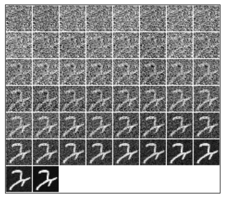
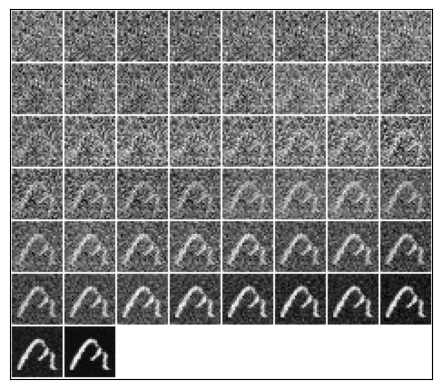
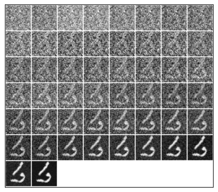
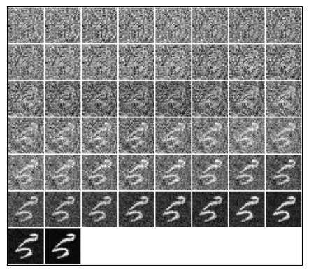
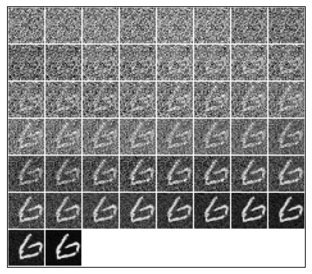
Each row above is a single denoising trajectory. Reading from left to right:
Qualitatively, the samples have the right kind of structure – clean strokes on a uniform background, broadly the shapes of MNIST digits, with stroke thickness and slant that vary between samples in the way real MNIST data varies. They are not perfect: a small DDPM trained for only three epochs with T = 50 leaves some artefacts (e.g. occasional in-between digits whose identity is ambiguous), but the overall behaviour confirms that the implementation is correct end-to-end.
ddim U-Net. Building the time-conditional U-Net from scratch was the largest single engineering chunk; basing it on the well-vetted ermongroup/ddim reference avoided a class of subtle indexing/conditioning bugs.temb and train on (image, label) pairs to generate a specific requested digit. With classifier-free guidance this also gives a single knob to trade off sample diversity for fidelity.ermongroup/ddim.